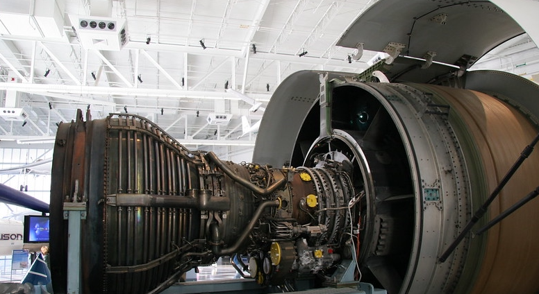
Expensive and critical equipment such as commercial jet engines are nowadays equipped with sensors that collect condition monitoring sensor data. We can use this data to build models that estimate the remaining useful life (RUL) of these equipment. Using these estimates, equipment with low estimated RUL can then be serviced or replaced before a catastrophic failure occurs.
In this project we will use the Commercial Modular Aero-Propulsion System Simulation (CMAPSS) data set to estimate the remaining useful life (RUL) of each engine units.
The data set consists of a set of timeseries sensor reading values for each engine unit for each flight. We will be training a regression machine learning model that takes in the sensor reading values as input features and produce an estimated remaining life cycle count of the engine.
We will be using root-mean-square error (RMSE) to measure the accuracy of our model. RMSE is given by the following equation:
where y is the actual RUL in units of engine cycles and y_hat is the predicted RUL value.
import os
import h5py
import time
import math
import random

import numpy as np
import pandas as pd
from pandas import DataFrame

import xgboost as xgb

import matplotlib.pyplot as plt
from matplotlib import gridspec
%matplotlib inline

from sklearn.preprocessing import StandardScaler
random.seed(13)
np.random.seed(13)
We will use the prognostics benchmark data set, N-CMPASS, prepared by Arias Chao, M et al [3]. The data set contains collections of multivariate timeseries sensor readings for a set of turbofan engines in various flight conditions. The entire data set contains 8 such collections, but during the project implementation, we will focus on only one collection due to time constraint. Each collection is in Hierarchical Data Format version 5, or .h5 file format.
For example, the dataset number 2 in the collection contains the following. The input timeseries contain 14 sensor readings, 4 flight scenario related variables, and 4 auxiliary variables for 9 different turbofan units. The entire timeseries is 6.5M time stamps long. The target variable is Remaining Useful Life (RUL) in units of engine cycles. Using the multivariate sensor reading data, target variable RUL can be predicted.
The data set size is in zipped file format around 15 GB and can be downloaded at https://ti.arc.nasa.gov/tech/dash/groups/pcoe/prognostic-data-repository/, under the section Turbofan Engine Degradation Simulation Data Set-2.
def load_data(file_name):
    with h5py.File(file_name, 'r') as hdf:
        # Development set
        W_dev = np.array(hdf.get('W_dev'))             # W
        X_s_dev = np.array(hdf.get('X_s_dev'))         # X_s
        Y_dev = np.array(hdf.get('Y_dev'))             # RUL
        A_dev = np.array(hdf.get('A_dev'))             # Auxiliary

        # Test set
        W_test = np.array(hdf.get('W_test'))           # W
        X_s_test = np.array(hdf.get('X_s_test'))       # X_s
        Y_test = np.array(hdf.get('Y_test'))           # RUL
        A_test = np.array(hdf.get('A_test'))           # Auxiliary

        # Variable names
        W_var = np.array(hdf.get('W_var'))
        X_s_var = np.array(hdf.get('X_s_var'))
        A_var = np.array(hdf.get('A_var'))
        W_var = list(np.array(W_var, dtype='str'))
        X_s_var = list(np.array(X_s_var, dtype='str'))
        A_var = list(np.array(A_var, dtype='str'))

    column_names = {
        'X_s_var' : X_s_var,
        'W_var' : W_var,
        'A_var' : A_var
    }
    df_dev = pd.DataFrame(np.concatenate((X_s_dev, W_dev, A_dev, Y_dev), axis = 1), columns = X_s_var + W_var + A_var + ['y'])
    df_test = pd.DataFrame(np.concatenate((X_s_test, W_test, A_test, Y_test), axis = 1), columns = X_s_var + W_var + A_var + ['y'])

    df_dev.columns = df_dev.columns.astype('str')
    df_dev = df_dev.astype({'unit': 'int32'})
    df_dev = df_dev.astype({'cycle': 'int32'})
    df_dev = df_dev.astype({'Fc': 'int32'})

    df_test.columns = df_test.columns.astype('str')
    df_test = df_test.astype({'unit': 'int32'})
    df_test = df_test.astype({'cycle': 'int32'})
    df_test = df_test.astype({'Fc': 'int32'})

    # Delete temp arrays to save memory
    del X_s_dev
    del W_dev
    del X_s_test
    del W_test

    return (df_dev, df_test, A_dev, A_test, column_names)
df_dev, df_test, A_dev, A_test, column_names = load_data('data_set/N-CMAPSS_DS02-006.h5')
We will first explore how many flights in total are in the development and test datasets.
df_dev[['unit','cycle']].groupby(['unit'], as_index=False).max()
| unit | cycle | |
|---|---|---|
| 0 | 2 | 75 |
| 1 | 5 | 89 |
| 2 | 10 | 82 |
| 3 | 16 | 63 |
| 4 | 18 | 71 |
| 5 | 20 | 66 |
In the development data set, we observe that a total of 6 Engine units (Unit 2, 5, 10, 16, 18 and 20) are flown between 63 cycles and 89 cycles. A total of 446 cycles are available in the development data set.
df_test[['unit','cycle']].groupby(['unit'], as_index=False).max()
| unit | cycle | |
|---|---|---|
| 0 | 11 | 59 |
| 1 | 14 | 76 |
| 2 | 15 | 67 |
In the test data set, we see three engine units (Unit 11, 14 and 15) are flown between 59 to 76 cycles each.
Now we will plot a typical flight profile.
# We plot the altitude and speed of the unit
def plot_flight_profile(data, unit, cycle):
    flight = data[(data.unit == unit) & (data.cycle == cycle)].reset_index()

    fig, (alt_plot, speed_plot) = plt.subplots(1, 2, figsize=(12,5))
    fig.suptitle(f"Unit {int(unit)} - Cycle {int(cycle)} - {len(flight)} Total flight data points")

    alt_plot.plot(flight.alt)
    alt_plot.title.set_text("Altitude")

    # Errors
    speed_plot.plot(flight.Mach)
    speed_plot.title.set_text("Speed (Mach)")
plot_flight_profile(df_dev, 10, 1)

We observe the aircraft climbing to altitute of around 30,000 feet and cruised at speed more than 0.7 mach, which is typical for a commerical jet aircaft.
Here we also note, that each sensor reading is taken every second, so total flight data points of 11764 corresponds to 11764 seconds or 3.2 hours.
Next, we explore the various sensor readings. The data set contains measurements (x_s) and virtual sensor measurements (X_v) for each time step. For this analysis, we will be using only the actual measurable senor readings (x_s), as virtual sensor readings will not be availble in real world setting.
print(f"The sensors in the data set are {column_names['X_s_var']}")
The sensors in the data set are ['T24', 'T30', 'T48', 'T50', 'P15', 'P2', 'P21', 'P24', 'Ps30', 'P40', 'P50', 'Nf', 'Nc', 'Wf']
The definition of the sensors are given as following by Arias Chao, M et al.

and the location of the sensors in the engine are shown below in the same paper

We will box plot each sensor reading and compare between a unit with high RUL and a unit with Low RUL.
def plot_compare_sensor(data, sensor_columns):
    high_rul_unit = data[data['y'] > 50] # More than 50 cycles remaining useful life
    low_rul_unit = data[data['y'] < 5] # Fewer than 5 cycles remaining

    fig, _ = plt.subplots(7, 2, figsize=(12,30))
    #fig.suptitle("Sensor Values")

    for i, ax in enumerate(fig.axes):
        ax.boxplot([high_rul_unit[sensor_columns[i]], low_rul_unit[sensor_columns[i]]], showfliers=False, labels=['High RUL', 'Low RUL'])
        ax.title.set_text(f"{sensor_columns[i]}")
plot_compare_sensor(df_dev, column_names['X_s_var'])

From the aggregate sensor readings alone, we will not be able to distinguish well between high RUL engines and low RUL engines.
Next, we will use a gradient boosted decision tree to get a baseline prediction.
X_dev = df_dev[column_names['X_s_var'] + column_names['W_var']]
y_dev = df_dev['y']

X_test = df_test[column_names['X_s_var'] + column_names['W_var']]
y_test = df_test['y']

dtrain = xgb.DMatrix(X_dev, label = y_dev)
dtest = xgb.DMatrix(X_test)
param = {
    'max_depth': 12,
    'eta':0.1,
    'objective':'reg:squarederror'
}

num_boost_round = 100

bst = xgb.train(param, dtrain, num_boost_round)
y_pred = bst.predict(dtest)
def rmse(y, y_pred):
    return np.sqrt(np.mean((y - y_pred)**2))
rmse(y_test, y_pred)
8.749051872719608
We obtain a benchmark model RMSE of 8.75 using the gradient boosted model.
xgb.plot_importance(bst)
<AxesSubplot:title={'center':'Feature importance'}, xlabel='F score', ylabel='Features'>

Next we proceed to model using a more complex model such as 1 Dimensional CNN.
Explanation of how 1D CNN works
For the input into 1DCNN network, we will first need to prepare the input data to have a fixed length.
class CMAPSSDataset(Dataset):
    def __init__(self, training_data):
        self.training_data = training_data

    def __len__(self):
        return len(self.training_data)

    def __getitem__(self, idx):
        return np.transpose(self.training_data[idx][0]).astype(np.float32), self.training_data[idx][1].astype(np.float32)
def groupby_unit_and_cycle(df, unit, cycle):
    # For each unit and cycle, get the sensor and W readings
    X_s_uc_sensor = df[(df.unit == unit) & (df.cycle == cycle)][column_names['X_s_var'] + column_names['W_var']]
    y_uc = df[(df.unit == unit) & (df.cycle == cycle)]['y']

    X_s_uc = pd.concat([X_s_uc_sensor, y_uc], axis=1)
    return X_s_uc

flights_dev = []
for unit in df_dev.unit.unique():
    for cycle in df_dev[df_dev.unit == unit]['cycle'].unique():
        flights_dev.append(groupby_unit_and_cycle(df_dev, unit, cycle))

flights_test = []
for unit in df_test.unit.unique():
    for cycle in df_test[df_test.unit == unit]['cycle'].unique():
        flights_test.append(groupby_unit_and_cycle(df_test, unit, cycle))

# Fit the Standard Scaler
scaler = StandardScaler()
scaler.fit(pd.concat(flights_dev, axis = 0).drop('y', axis = 1))

print(f'Dev Data Set Flights: {len(flights_dev)}')
print(f'Test Data Set Flights: {len(flights_test)}')
Dev Data Set Flights: 446
Test Data Set Flights: 202
# Define the input length
input_length = 100

# Define the validation data percent
val_data_percent = 0.05 # 5 percent
def create_fixed_length_data(X, y, input_length = 100):
    data = []
    i = 0
    while True:
        truncated_X = X[i * int(input_length/2): i * int(input_length/2) + input_length] # Take first n seconds
        if truncated_X.shape[0] < input_length:
            truncated_X = X[-input_length:]
            data.append((truncated_X, y.iloc[0]))
            break
        data.append((truncated_X, y.iloc[0]))
        i += 1
    return data
train_data = []
val_data = []

for flight in flights_dev:
    flight_y = flight['y']
    flight_x = scaler.transform(flight.drop('y', axis=1))
    fixed_length_data = create_fixed_length_data(flight_x, flight_y, input_length)
    if random.random() >= val_data_percent:
        train_data += fixed_length_data
    else:
        val_data += fixed_length_data

print(f'Total training flight segments: {len(train_data)}')
print(f'Total validation flight segments: {len(val_data)}')
Total training flight segments: 99683
Total validation flight segments: 5381
cmapss_train_dataset = CMAPSSDataset(train_data)
cmapss_val_dataset = CMAPSSDataset(val_data)
train_dataloader = DataLoader(cmapss_train_dataset, batch_size=100, shuffle=True)
val_dataloader = DataLoader(cmapss_val_dataset, batch_size=100, shuffle=True)
cmapss_train_dataset[0][0].shape
(18, 100)
class CMAPSS1DCNN(nn.Module):
    def __init__(self, input_channels, input_length, hyper_params):
        super(CMAPSS1DCNN, self).__init__()

        self.one_by_one_conv = nn.Sequential(
            nn.Conv1d(input_channels, input_channels, 1),
            nn.ReLU())

        self.conv_layers = nn.ModuleList(
            [nn.Sequential(
                nn.Conv1d(input_channels, input_channels, hyper_params['conv_kernel_size'], padding = int((hyper_params['conv_kernel_size'] - 1) / 2)),
                nn.ReLU()) for i in range(hyper_params['num_conv_layers'])]
        )

        self.flatten = nn.Flatten()

        self.linear_relu_stack = nn.Sequential(
              nn.Linear(input_channels * input_length, hyper_params['linear_layer_size']),
              nn.Tanh(),
              nn.Linear(hyper_params['linear_layer_size'], 1))

    def forward(self, x):
        residual = self.one_by_one_conv(x)
        y = residual

        for i, conv_layer in enumerate(self.conv_layers):
            y = conv_layer(y) + residual

        y = self.flatten(y)
        y = self.linear_relu_stack(y)
        return torch.squeeze(y)
# Add RayTune Library here to parallely tune hyper parameters
# Add Wandb
hyper_params = {
    'num_conv_layers' : 6,
    'linear_layer_size': 500,
    'conv_kernel_size': 3
}

input_channels = cmapss_train_dataset[0][0].shape[0]
input_length = cmapss_train_dataset[0][0].shape[1]

cnn_model = CMAPSS1DCNN(input_channels, input_length, hyper_params = hyper_params)
cnn_model.to(device)

print(cnn_model)
CMAPSS1DCNN(
  (one_by_one_conv): Sequential(
    (0): Conv1d(18, 18, kernel_size=(1,), stride=(1,))
    (1): ReLU()
  )
  (conv_layers): ModuleList(
    (0): Sequential(
      (0): Conv1d(18, 18, kernel_size=(3,), stride=(1,), padding=(1,))
      (1): ReLU()
    )
    (1): Sequential(
      (0): Conv1d(18, 18, kernel_size=(3,), stride=(1,), padding=(1,))
      (1): ReLU()
    )
    (2): Sequential(
      (0): Conv1d(18, 18, kernel_size=(3,), stride=(1,), padding=(1,))
      (1): ReLU()
    )
    (3): Sequential(
      (0): Conv1d(18, 18, kernel_size=(3,), stride=(1,), padding=(1,))
      (1): ReLU()
    )
    (4): Sequential(
      (0): Conv1d(18, 18, kernel_size=(3,), stride=(1,), padding=(1,))
      (1): ReLU()
    )
    (5): Sequential(
      (0): Conv1d(18, 18, kernel_size=(3,), stride=(1,), padding=(1,))
      (1): ReLU()
    )
  )
  (flatten): Flatten(start_dim=1, end_dim=-1)
  (linear_relu_stack): Sequential(
    (0): Linear(in_features=1800, out_features=500, bias=True)
    (1): Tanh()
    (2): Linear(in_features=500, out_features=1, bias=True)
  )
)
# Change here for CNN vs LSTM
model = cnn_model
def train_loop(dataloader, model, loss_fn, optimizer):
    size = len(dataloader.dataset)
    num_batches = len(dataloader)
    train_loss = 0
    for batch, (X, y) in enumerate(dataloader):
        # Compute prediction and loss
        X = X.to(device)
        y = y.to(device)
        pred = model(X)
        loss = loss_fn(pred, y)
        train_loss += loss.item()

        # Backpropagation
        optimizer.zero_grad()
        loss.backward()
        optimizer.step()
    train_loss /= num_batches
    print(f"Train Avg loss: {train_loss:>8f} \n")

def val_loop(dataloader, model, loss_fn):
    size = len(dataloader.dataset)
    num_batches = len(dataloader)
    val_loss = 0
    error = 0

    with torch.no_grad():
        for X, y in dataloader:
            X = X.to(device)
            y = y.to(device)
            pred = model(X)
            val_loss += loss_fn(pred, y).item()
            error += torch.square(y - pred).sum()

    val_loss /= num_batches
    val_rmse = math.sqrt (error / size)
    print(f"Val Error: \n RMSE: {val_rmse:>8f}, Val Avg loss: {val_loss:>8f} \n")
loss_function = nn.MSELoss()
alpha_zero = 1e-3
lr_decay_rate = 0.05
optimizer = torch.optim.Adam(model.parameters(), lr=alpha_zero, weight_decay = 0.0)

start_time = time.time()
epochs = 20

for epoch in range(epochs):
    # Learning rate decay
    lr = alpha_zero / (1 + lr_decay_rate * epoch)
    optimizer.param_groups[0]['lr'] = lr

    print(f"Epoch {epoch}\n-------------------------------")
    train_loop(train_dataloader, model, loss_function, optimizer)
    val_loop(val_dataloader, model, loss_function)

print("Done!")
print("--- %s seconds ---" % (time.time() - start_time))
Epoch 0
-------------------------------
Train Avg loss: 526.658233

Val Error:
 RMSE: 24.791911, Val Avg loss: 617.981371

Epoch 1
-------------------------------
Train Avg loss: 450.268984

Val Error:
 RMSE: 13.000874, Val Avg loss: 183.920892

Epoch 2
-------------------------------
Train Avg loss: 71.517646

Val Error:
 RMSE: 6.462801, Val Avg loss: 40.414214

Epoch 3
-------------------------------
Train Avg loss: 51.464455

Val Error:
 RMSE: 7.363230, Val Avg loss: 52.876593

Epoch 4
-------------------------------
Train Avg loss: 48.501946

Val Error:
 RMSE: 6.721429, Val Avg loss: 44.987722

Epoch 5
-------------------------------
Train Avg loss: 43.767271

Val Error:
 RMSE: 6.564008, Val Avg loss: 42.098041

Epoch 6
-------------------------------
Train Avg loss: 44.900655

Val Error:
 RMSE: 6.955630, Val Avg loss: 47.673742

Epoch 7
-------------------------------
Train Avg loss: 43.172047

Val Error:
 RMSE: 7.796412, Val Avg loss: 59.687594

Epoch 8
-------------------------------
Train Avg loss: 42.247078

Val Error:
 RMSE: 6.326452, Val Avg loss: 39.857030

Epoch 9
-------------------------------
Train Avg loss: 41.959968

Val Error:
 RMSE: 6.360924, Val Avg loss: 40.485428

Epoch 10
-------------------------------
Train Avg loss: 41.990871

Val Error:
 RMSE: 6.341487, Val Avg loss: 43.687218

Epoch 11
-------------------------------
Train Avg loss: 40.821624

Val Error:
 RMSE: 5.961547, Val Avg loss: 34.723103

Epoch 12
-------------------------------
Train Avg loss: 39.941932

Val Error:
 RMSE: 6.217217, Val Avg loss: 40.964421

Epoch 13
-------------------------------
Train Avg loss: 39.640183

Val Error:
 RMSE: 6.840417, Val Avg loss: 45.556415

Epoch 14
-------------------------------
Train Avg loss: 39.703224

Val Error:
 RMSE: 6.162441, Val Avg loss: 36.923182

Epoch 15
-------------------------------
Train Avg loss: 39.278862

Val Error:
 RMSE: 6.341795, Val Avg loss: 42.118928

Epoch 16
-------------------------------
Train Avg loss: 38.202816

Val Error:
 RMSE: 5.808239, Val Avg loss: 32.768902

Epoch 17
-------------------------------
Train Avg loss: 37.914707

Val Error:
 RMSE: 6.034233, Val Avg loss: 35.665258

Epoch 18
-------------------------------
Train Avg loss: 39.325867

Val Error:
 RMSE: 5.858417, Val Avg loss: 35.263573

Epoch 19
-------------------------------
Train Avg loss: 37.602668

Val Error:
 RMSE: 6.298915, Val Avg loss: 39.675915

Done!
--- 1763.282726764679 seconds ---
# Set the model to eval mode
model.eval()
for flight in flights_test:
    flight_y = flight['y'].iloc[0]
    # this is so that it can be scored multiple times
    flight_x = scaler.transform(flight.drop(['y', 'y_pred'], axis=1, errors='ignore'))
    y_partial_preds = []

    i = 0
    break_loop = False
    while True:
        truncated_X = flight_x[i * int(input_length/2) : i * int(input_length/2) + input_length]

        if truncated_X.shape[0] < input_length:
            truncated_X = flight_x[-input_length:]
            break_loop = True

        with torch.no_grad():
            X_input = torch.from_numpy(np.transpose(truncated_X).astype(np.float32))
            X_input = X_input.to(device)
            X_input = torch.unsqueeze(X_input, 0)
            pred = model(X_input)
            y_partial_preds.append(pred.item())

        if break_loop:
            break
        i += 1

    y_pred = sum(y_partial_preds)/len(y_partial_preds)
    flight['y_pred'] = y_pred
flights_test_df = pd.concat(flights_test, axis = 0)
# Put back the flight information for further analysis
A_test_df = pd.DataFrame(A_test, columns = column_names['A_var'])
flights_test_df = pd.concat((flights_test_df, A_test_df), axis = 1)
test_flight_summary = flights_test_df.groupby(['unit', 'cycle', 'hs'], as_index = False)[['y','y_pred']].mean()
test_flight_summary['error'] = test_flight_summary['y'] - test_flight_summary['y_pred']
test_flight_summary['error_squared'] = test_flight_summary['error']**2
rmse_test = math.sqrt(sum(test_flight_summary['error_squared'])/len(test_flight_summary))
print(f'RMSE for the test data is {rmse_test}')
6.376264294260416
def plot_RUL(df, unit):

    fig, (pred_plot, error_plot) = plt.subplots(1, 2, figsize=(12,5))
    fig.suptitle(f"Unit {int(unit)}")

    # Pred vs Y
    pred_plot.plot(df.cycle, df.y)
    pred_plot.plot(df.cycle, df.y_pred)
    pred_plot.title.set_text("Prediction vs Actual RUL")

    # Errors
    error_plot.plot(df.cycle, df.error, 'r')
    hs_plot = error_plot.twinx()
    hs_plot.plot(df.cycle, df.hs, 'b+', alpha=.5)
    error_plot.title.set_text("Error")
for test_unit in test_flight_summary.unit.unique():
    plot_RUL(test_flight_summary[test_flight_summary.unit == test_unit], test_unit)


We observe that the CNN model does has higher error distribution when the engines are performing well, and lower errors when the engines start to develop health issues.
# TODO: Discussion of Result
# TODO: Further research - digital twins